
MATH 316 — Applied Ordinary Differential Equations
University of New Mexico · 3 credit hours
An introduction to ordinary differential equations, their analytical solutions, and models of phenomena in the physical and natural sciences.
This is a semester-independent course overview. Official meeting times, assessment details, and policies are specified separately for each offering.
Course syllabus
1. Course information
Course: MATH 316 — Applied Ordinary Differential Equations
Institution: University of New Mexico
Credits: 3
The course emphasizes how differential equations arise from models, how their solutions are constructed, and how solution behavior can be understood qualitatively.
2. Learning objectives
By the end of the course, students should be able to:
- Recognize and solve separable and first-order linear differential equations.
- Interpret direction fields, equilibria, autonomous equations, and stability.
- Construct and analyze simple mathematical models, including population and spring–mass systems.
- Solve second-order linear equations using characteristic roots and undetermined coefficients.
- Use Laplace transforms to solve initial-value problems with continuous, piecewise, and impulsive forcing.
- Solve two-dimensional linear systems using eigenvalues and eigenvectors, and sketch phase portraits.
- Analyze equilibria and local behavior in selected nonlinear systems.
3. Course materials and prerequisites
Prerequisite: MATH 1522 (Calculus II). Calculus III may be taken before or concurrently, subject to the current UNM course requirements.
Textbook: J. David Logan, A First Course in Differential Equations, 3rd edition (textbook from a recent coordinated offering).
Course resources: Notes, weekly assignments, announcements, and grades are distributed through UNM Canvas for each semester.
4. Assessment and grading
The following is a representative grading breakdown, not a promise that future offerings will use the same weights.
| Assessment | Weight |
|---|---|
| Weekly homework | 14% |
| Instructor discretion / participation | 4% |
| Four midterm exams | 60% |
| Cumulative final exam | 22% |
Homework: Regular written assignments provide practice with solution methods and modeling. Solutions should be legible, logically organized, and submitted according to the current course instructions.
Exams: Timed written exams evaluate solution techniques, conceptual reasoning, and interpretation. The final exam is cumulative. Exact examination dates, permitted materials, grading rules, and any dropped scores are semester-specific.
5. General course schedule
Topics are presented in teaching order, without tying the outline to any particular semester.
| Order | Topic |
|---|---|
| 1 | First-order differential equations |
| 2 | Second-order linear differential equations |
| 3 | Laplace transforms |
| 4 | Linear systems of differential equations |
| 5 | Nonlinear systems and applications |
Lecture materials
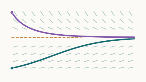
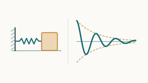
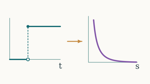
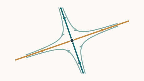
Lecture notes are arranged sequentially by chapter. Each chapter has an illustration, and available lecture notes link to PDFs.
1. First-order differential equations
First-order solution techniques, direction fields, equilibrium behavior, and mathematical models.
Introduction to first-order differential equations
What differential equations model and how first-order equations are classified.
Solutions and direction fields
Understanding solution curves and the information contained in direction fields.
Separation of variables
Solving separable equations by integrating functions of one variable.
Linear equations and integrating factors
Solving linear first-order equations using an integrating factor.
Applications of first-order equations
Building and interpreting mathematical models from first-order equations.
Autonomous equations and stability
Finding equilibria and classifying stability in autonomous equations.
Population models
Using differential equations to model population growth and competition.
Existence and uniqueness
Determining when an initial-value problem has a unique local solution.
2. Second-order linear differential equations
Characteristic equations, forced and unforced oscillations, and spring–mass systems.
Spring–mass models
Deriving a differential-equation model for spring–mass motion.
Distinct real characteristic roots
Solving homogeneous equations with distinct real characteristic roots.
Repeated characteristic roots
Solving homogeneous equations with repeated characteristic roots.
Complex characteristic roots
Interpreting complex roots and oscillatory solutions.
Unforced spring–mass systems
Classifying undamped, underdamped, critically damped, and overdamped motion.
Method of undetermined coefficients
Finding particular solutions by the method of undetermined coefficients.
Forced spring–mass systems
Analyzing forced oscillations, beats, and resonance.
3. Laplace transforms
Transforms of elementary functions, initial-value problems, step functions, and impulses.
Definition and basic properties of the Laplace transform
Introducing the Laplace integral transform and its basic properties.
Solving initial-value problems
Solving initial-value problems with Laplace transforms.
Shift theorems
Applying first and second shifting properties.
Heaviside step function
Representing discontinuous inputs using the Heaviside step function.
Piecewise forcing
Modeling piecewise forcing functions and solving the resulting equations.
Impulse forces
Understanding impulse forcing and its effect on solutions.
4. Linear systems of differential equations
Matrix methods, eigenvalues and eigenvectors, and the geometry of two-dimensional phase portraits.
Matrix formulation and eigenvectors
Representing first-order systems in matrix form and computing eigensolutions.
Phase portraits and stability
Sketching saddle, node, spiral, and center trajectories.
Repeated and zero eigenvalues
Analyzing special eigenvalue cases in linear systems.
5. Nonlinear systems and applications
Equilibria, linearization, and nonlinear models such as predator–prey dynamics.

From higher-order equations to systems
Rewriting scalar differential equations as first-order systems.
Equilibria and linearization
Understanding local dynamics near stationary points.
Competing species and predator–prey models
Studying interacting populations using nonlinear models.
Nonlinear pendulum
Examining nonlinear motion and phase portraits.
Interactive tools
Linear Systems Explorer — Plot direction fields for x′ = Ax, change the matrix, and click to trace solution trajectories. Includes sample portraits, eigenvalues, and real eigendirections.
Nonlinear Systems Explorer — Enter two functions, explore direction fields and nullclines, and click to trace trajectories. Includes pendulum, saddle and spiral, and saddle and node examples.
Pendulum Simulator — Animate a pendulum alongside its phase-plane trajectory and angle-versus-time plot. Compare damping presets or choose your own initial conditions.