
MATH/CS 375 — Introduction to Numerical Computing
University of New Mexico · 3 credit hours
An introduction to numerical methods and scientific computing, with computational experiments and algorithm implementations in MATLAB.
This is a semester-independent course overview. Official meeting times, exam counts, grading details, and policies are set in the syllabus for each offering.
Course syllabus
1. Course information
Course: MATH/CS 375 — Introduction to Numerical Computing
Institution: University of New Mexico
Credits: 3
The course explores numerical algorithms for differentiation, root finding, linear systems, interpolation, integration, eigenvalue problems, approximation, and differential equations, with particular attention to convergence, stability, and computational cost.
2. Learning objectives
By the end of the course, students should be able to:
- Explain truncation error, rounding error, conditioning, and convergence of numerical approximations.
- Implement numerical algorithms in MATLAB and evaluate their accuracy and computational cost.
- Solve linear systems using direct and iterative techniques, and understand when each is appropriate.
- Apply root-finding methods to nonlinear equations and compare convergence behavior.
- Construct interpolating polynomials and splines and assess approximation errors.
- Approximate derivatives and integrals using numerical formulas.
- Use numerical techniques for eigenvalue problems, least-squares approximation, and initial-value problems.
3. Course materials and prerequisites
Prerequisites: MATH 2531 (Calculus III) and CS 261 (Mathematical Foundations of Computer Science), as listed in the Spring 2026 course syllabus. Background in programming and differential equations is helpful.
Textbook: Ward Cheney and David Kincaid, Numerical Mathematics and Computing, 7th edition (6th edition also suitable for the referenced offering).
Software: MATLAB is used for algorithm implementation, experiments, and written computational assignments.
Course resources: Slide PDFs, assignments, announcements, and grades are provided through UNM Canvas.
4. Assessment and grading
The following illustrates the grading breakdown used in Spring 2026. The number and weight of midterm exams may vary between semesters.
| Assessment | Weight |
|---|---|
| Homework | 30% |
| Midterm exam 1 | 20% |
| Midterm exam 2 | 20% |
| Cumulative final exam | 30% |
Homework: Assignments combine mathematical derivations, numerical calculations, and MATLAB programming. Written reports, including appropriately labeled figures and code, are normally submitted as PDFs through Canvas.
Exams: Written exams assess numerical methods, mathematical reasoning, and the interpretation of numerical results. The final exam is cumulative; semester-specific exam rules are provided separately.
5. General course schedule
This schedule describes the order of major topics; exact pacing and assessment dates depend on the semester.
Lecture materials
The lectures below are organized sequentially by topic. Each entry includes a short description and a PDF of the slides, with one illustration space per topic group.
1. Numerical foundations
Course introduction
An overview of the course and the role of computation in numerical mathematics.
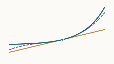
Taylor series and convergence
Using Taylor expansions to study approximations and convergence.
Introduction to floating-point numbers
How real numbers are represented with finite-precision floating-point numbers.
Floating-point arithmetic
How rounding affects computations and the accuracy of numerical results.
2. Numerical differentiation
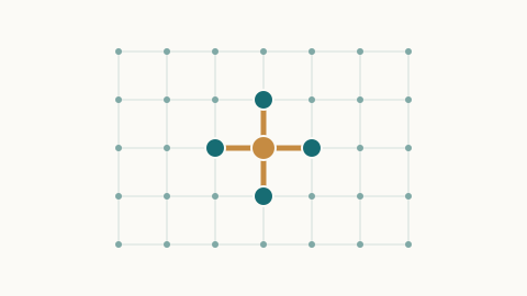
Approximating derivatives and improving accuracy through extrapolation.
Numerical differentiation
Approximating derivatives numerically and understanding sources of error.
Extrapolation
Using extrapolation to improve the accuracy of numerical approximations.
3. Solving nonlinear equations
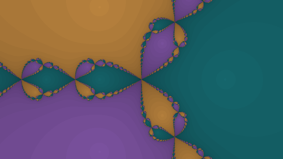
Finding roots numerically and comparing methods for solving nonlinear problems.
Nonlinear equations and the bisection method
Finding solutions of nonlinear equations with bracket-based methods.
Newton Method
Finding roots with the Newton method.
Secant method
Using the secant method to approximate roots without derivatives.
4. Direct methods for linear systems
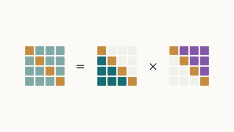
Solving matrix equations using elimination and factorizations, with attention to computational cost and numerical stability.
Linear algebra fundamentals
Matrix and vector ideas that underlie numerical linear algebra.
Counting operations and solving special systems
Estimating computational cost and using structure to solve special systems.
Gaussian elimination
Solving systems of linear equations using Gaussian elimination.
Gaussian elimination (continued)
Continuing the elimination process and its practical implementation.
Numerical stability
Understanding stability and the effects of rounding in linear systems.
LU factorization
Factoring a matrix into triangular factors for efficient solution methods.
LDL and Cholesky factorizations
Using matrix factorizations for symmetric linear systems.
5. Iterative methods for linear systems
Solving linear systems by repeated approximation, including methods that exploit sparse matrices.
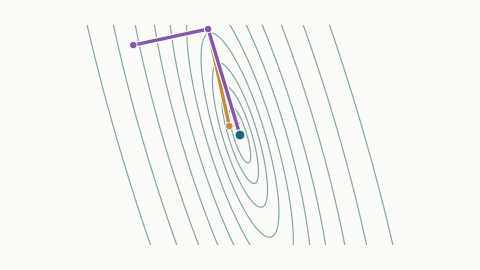
Stationary iterative methods
Approximating solutions of linear systems using repeated iterations.
Sparsity and iterative methods
Taking advantage of sparse matrices in iterative computations.
Iterative methods (continued)
Further properties and applications of iterative methods.
6. Polynomial interpolation
Constructing interpolating polynomials and understanding the errors they introduce.
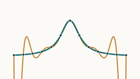
Polynomial interpolation
Constructing polynomials that interpolate a given set of data points.
Newton interpolation
Writing interpolating polynomials in Newton form.
Interpolation error
Understanding how interpolation error depends on the data and method.
7. Splines and data interpolation
Using piecewise polynomials and MATLAB tools to interpolate and visualize data.

Splines
Using piecewise polynomials to build smooth interpolants.
Interpolation, splines, and data visualization in MATLAB
Working with interpolation, splines, and three-dimensional data in MATLAB.
8. Numerical integration
Approximating integrals using Newton–Cotes formulas and Gaussian quadrature.
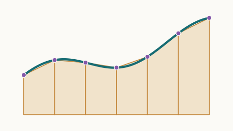
Numerical integration
Approximating definite integrals using sampled function values.
Newton–Cotes formulas
Studying numerical integration formulas based on interpolating polynomials.
Gaussian quadrature
Choosing quadrature nodes and weights for greater accuracy.
Generalized Gaussian quadrature
Extending Gaussian quadrature to more general integration settings.
9. Eigenvalue methods and Markov chains
Computing eigenpairs and applying matrix methods to Markov chains.
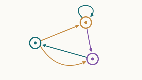
Power method
Using the power method to approximate an eigenvalue and eigenvector.
Markov chains
Studying Markov chains through matrix-based computation.
10. Least-squares approximation
Fitting models to data when an exact fit is unavailable or undesirable.

Least-squares methods
Finding approximate models that fit more data than an exact system can.
Least squares
Solving and interpreting least-squares problems.
11. Numerical methods for differential equations
Approximating solutions of initial-value problems with time-stepping schemes.
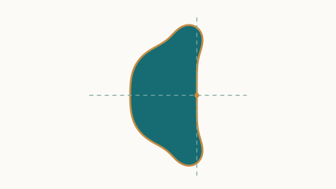
Numerical methods for differential equations
Approximating solutions to differential equations using numerical methods.
Numerical methods for differential equations (continued)
Exploring further numerical methods for differential equations.
Runge–Kutta methods
Improving solution accuracy with Runge–Kutta time-stepping methods.
12. Monte Carlo simulation
Estimating quantities through random sampling and computational experiments.
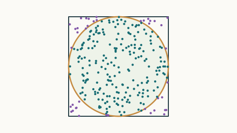
Monte Carlo methods
Estimating quantities using random sampling and Monte Carlo simulation.